Software
Software is a program for a computer.
A program is a sequence of coded instructions that can be inserted into a computer.
We distinguish two types of software:
- System software: operating systems, device drivers, and utilities.
- Application software: productivity software, graphics software, databases, browsers, games, and the like.
System software is essential for the functioning of a general-purpose computer, managing hardware and providing a platform on which application software runs. System software provides value to the end user indirectly, through application software.
Most of what follows should be applicable to both categories. In case of conflict, however, we’ll focus on application software, because the majority of software falls into that bucket.
In summary, software consists of instructions for a computer that tell it what to compute. Let’s look at the science of computing next.
Computing
Automata theory is the study of abstract computing devices, named machines or automata [Hopcroft2007]. The theory formally defines different types of automata and derives mathematical proofs about them.
Finite automata
The simplest types of automata are finite automata. Formally, a Deterministic Finite Automaton (DFA) is a tuple , where
- is a finite set of states the automaton can be in.
- is a finite set of symbols, called the input alphabet of the automaton.
- is the transition function mapping states to successor states while consuming input.
- is the start state.
- is the set of accepting states.
We can visually present a DFA using a transition diagram. For instance, the DFA may look like this for a suitable :
stateDiagram-v2
  direction LR
  [*] --> p
  p --> p: 1
  p --> q: 0
  q --> q: 0
  q --> r: 1
  r --> r: 0,1
  r --> [*]
An alternative description of a DFA uses a table format. A transition table shows inputs as rows, the current states as columns, and next states in the intersection of the two. For example, the PDA above looks like this:
| p | q | r | |
|---|---|---|---|
| 0 | q | q | r |
| 1 | p | r | r |
Let be a word made up of symbols such that . If there are transitions in such that , , etc. and , then accepts . The set of all words that accepts is the language of , .
For instance, the language of the automaton above is the set of strings composed of s and s that contain the substring .
Languages accepted by DFAs are regular languages. Regular languages have many applications in software. For instance, they describe keywords and valid identifiers in programming languages or the structure of a URL. They’re also useful in searching documents and describing protocols.
A Nondeterministic Finite Automaton (NFA) is like a DFA, except returns a subset of rather than a single state. In other words, an NFA can be in more than one state at the same time. It’s possible to convert an NFA to a DFA, so the languages accepted by NFAs are also regular languages.
An -NFA is an NFA with the extra feature that it can transition on , the empty string. In other words, an -NFA can make transitions without consuming input. It’s possible to convert an -NFA to a DFA as well, so the languages accepted by -NFAs are also regular languages.
Regular expressions are an alternative way of describing regular languages. They use the symbols of along with the operators (union) and (zero or more times) and parentheses. For instance, the regular expression defines the same language as the PDA above. We can convert regular expressions to DFAs and vice versa.
Regular languages can describe parts of programs, but not entire programs. The memory of a DFA is too limited, since it consists of a finite number of states. Let’s look at more powerful automata that define more useful languages.
Pushdown automata
A Pushdown Automaton (PDA) is an -NFA with a stack on which it can store information. A PDA can access information on the stack only in a first-in-first-out way. The stack allows the PDA to remember things, which makes it more powerful than a DFA. For instance, no DFA can recognize palindromes, but a PDA can.
Formally, a PDA is a tuple . We’ve seen most of these symbols already in the definition of DFAs. The new ones are:
- is the alphabet of stack symbols, the information that can go on the stack.
- is the initial symbol on the stack when the PDA starts.
The transition function is slightly different. It takes the current state, an input symbol, and the symbol from the top of the stack as input. It outputs pairs consisting of a new state and a string of stack symbols that replace the top of the stack.
- This stack string can be , the empty string, in which case pops an element off the stack.
- It can also be the same as the top of the stack, in which case the stack remains the same.
- Or it can be a different string, even consisting of multiple symbols. In that case, the PDA pops the top symbol off the stack and pushes the output string onto the stack, one symbol at a time.
We can visualize PDAs using transition diagrams, just like DFAs. The edges show both the input symbol consumed and the old and new top of the stack. For instance, an edge labeled between nodes and means that contains the pair . Here, , where .
A PDA can accept a word in two ways:
- By final state, like for finite automatons.
- By empty stack, which is a new capability compared to finite automatons. In this definition, when the PDA pops the last symbol off its stack, the input it consumed up to then is a word that it accepts.
These two ways of accepting words and thus defining a language turn out to be the same. Suppose a PDA accepts by final state the language . We can construct a different PDA that accepts by empty stack precisely . The converse is also true.
We call the languages accepted by PDAs the context-free languages. Context-free languages, like regular languages, have important applications in software development. Before we dive into those, let’s look at an alternative way to specify the context-free languages: context-free grammars.
A Context-Free Grammar (CFG), or just grammar, is a tuple , where
- is a set of variables. Each variable represents a language, or set of strings. Variables are building block for the bigger language that the grammar defines.
- is a set of terminals. A terminal is a symbol in the language the grammar defines.
- is a set of productions. A production is of the form , where is the head and is the body. A body consists of zero or more variables and terminals.
- is the start symbol.
For instance, a grammar for the palindromes over and is:
Where is the following set of productions:
We can derive a word from a CFG . Start with its start symbol, and recursively replace variables using the productions until only terminal symbols remain. The set of words we can derive from a grammar is its language, .
A parse tree is a tree representation of a derivation in a CFG . The root of this tree is the start symbol of . For some production , there is a child under parent and these children are in order.
Here’s an example parse tree for that derives the palindrome :
graph TB
  A[P]
  B[0]
  C[P]
  D[0]
  E[1]
  F[P]
  G[1]
  H[0]
  A --- B
  A --- C
  A --- D
  C --- E
  C --- F
  C --- G
  F --- H
The leaves from left to right spell the derived word.
Languages we can derive from CFGs are precisely the context-free languages. For every CFG that defines a language , we can construct a PDA such that . The converse is also true.
Context-free languages can recognize programming languages. A parse tree of a CFG for a programming language describes a single program in that language. For instance, here’s a fictitional parse tree for the infamous program in C:
graph TB
  Program --- Function --- Declaration --- TypeSpecifier --- int
  Function --- CompoundStatement --- Statement --- ExpressionStatement --- CallExpression --- Identifier --- printf
  CallExpression --- StringLiteral

  StringLiteral[""Hello, world!""]
We now have the vocabulary to describe the structure of a program and of programming languages. However, PDAs aren’t powerful enough to describe the runtime behavior of all but the simplest programs. Let’s next look at automata that can.
Turing machines
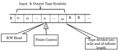
A Turing Machine (TM) is a generalization of a PDA where an infinite tape replaces the stack. This tape is a linear sequence of cells, one of which, the head, the TM points to. Initially, the input is on the tape, one symbol per cell, and the head points to the first input symbol. Left and right of the input, all cells are blank.
Formally, a TM is a tuple . We’ve seen most of these symbols already in the definition of previous automata. The new and changed ones are:
- is a set of tape symbols. These are analogous to the stack symbols of a PDA. Note that .
- is the blank symbol, where .
- The transition function takes a state and tape symbol as input. It produces a triple . Here is the next state. is the tape symbol written to the head. is the direction in which the head moves: = left and = right.
We can visualize TMs using transition diagrams, where edges are of the form . Here is the tape symbol at the head and is the replacement tape symbol. is the direction in which to move the head ( or ).
Several variations of TMs exist, such as those with multiple tapes or with the ability to keep the head in place. A non-deterministic variant exists as well. All these variations have the same power, in the sense that deterministic one-tape TMs can simulate them. Simpler models exists as well, like a PDA with two stacks, that can simulate a TM.
The languages TMs accept are the Recursively Enumerated (RE) languages. Like with the other types of languages, there are alternative models for expressing RE languages, for instance -calculus and general recursive functions. We call any model that accepts RE languages Turing-complete.
Real computers are Turing complete, if we assume the computer has access to an infinite number of disks of external storage. These disks simulate the TM’s infinite tape.
The Church-Turing thesis states that anything computable is computable by a TM. In other words, there can be no more powerful automata than TMs. Despite the lack of a formal proof, most people accept this thesis as true.
Programming a TM isn’t practical for solving real-world problems. The linear access model of a TM to its external storage, the tape, means the TM has to travel great distances. Real computers can access memory locations directly, which is much more efficient. Having said that, a TM is a useful abstraction to reason about computation.
Output
The transition function of an automaton gives the next state and, depending on the automaton, writes to external storage (stack or tape). We can change to also output something. A finite state machine that produces output is a transducer.
Conceptually, we can think of a transducer as a TM with two tapes: one for input and one for output. This implies that the output is a string of tape symbols from .
Output is often omitted in automata theory, which focuses on solving problems by accepting input. For real computer programs, however, output is crucial.
One may argue that the output of a TM is somewhere on its tape. This works for TMs and to some extent for PDAs, but not for DFAs. As we’ve seen, DFAs are useful in many situations in software development and some of those situations require output.
For instance, a tokenizer is a program that breaks a stream of text into individual tokens. These tokens may be part of a grammar, in which case we call the tokenizer a lexer or lexical analyzer. A program that analyzes text against a grammar and produces parse trees is a parser. The lexer must output the token it accepted, so that the parser can use it in its evaluations.
Model of software
Here’s a concept map of a software application based on automata theory:
graph
  Application --has--> State
  Application --allows--> Transition
  Transition --from/to --> State
  Transition --accepts--> Input
  Transition --produces--> Output
  Transition --reads from &\nwrites to --> ES[External storage]
This model is admittedly not super useful yet, but it’ll serve as the basis for later enhancements.
Now that we understand the basics of both software and engineering, let’s put these two together.